R for Data Analysis
Overview
Teaching: 150 min
Exercises: 15 minQuestions
How can I summarize my data in R?
How can R help make my research more reproducible?
How can I combine two datasets from different sources?
How can data tidying facilitate answering analysis questions?
Objectives
To become familiar with the functions of the
dplyrandtidyrpackages.To be able to use
dplyrandtidyrto prepare data for analysis.To be able to combine two different data sources using joins.
To be able to create plots and summary tables to answer analysis questions.
Contents
- Getting started
- An introduction to data analysis in R using
dplyr - Cleaning up data
- Joining data frames
- Analyzing combined data
- Finishing with Git and GitHub
Getting Started
First, navigate to the un-reports directory however you’d like and open un-report.Rproj.
This should open the un-report R project in RStudio.
You can check this by seeing if the Files in the bottom right of RStudio are the ones in your un-report directory.
Yesterday we spent a lot of time making plots in R using the ggplot2 package. Visualizing data using plots is a very powerful skill in R, but what if we would like to work with only a subset of our data? Or clean up messy data, calculate summary statistics, create a new variable, or join two datasets together? There are several different methods for doing this in R, and we will touch on a few today using functions the dplyr package.
First, we will create a new RScript file for our work. Open RStudio. Choose “File” > “New File” > “RScript”. We will save this file as un_data_analysis.R
Loading in the data
We will start by importing the complete gapminder dataset that we used yesterday into our fresh new R session. Yesterday we did this using a “point-and-click” commands. Today let’s type them into the console ourselves: gapminder_data <- read_csv("data/gapminder_data.csv")
Exercise
If we look in the console now, we’ll see we’ve received an error message saying that R “could not find the function
read_csv()”. Hint: Packages…Solution
What this means is that R cannot find the function we are trying to call. The reason for this usually is that we are trying to run a function from a package that we have not yet loaded. This is a very common error message that you will probably see a lot when using R. It’s important to remember that you will need to load any packages you want to use into R each time you start a new session. The
read_csvfunction comes from thereadrpackage which is included in thetidyversepackage so we will just load thetidyversepackage and run the import code again.
Now that we know what’s wrong, We will use the read_csv() function from the Tidyverse readr package. Load the tidyverse package and gapminder dataset using the code below.
library(tidyverse)
── Attaching packages ──────────────────────────────────────────────────────────────── tidyverse 1.3.1 ──
✔ ggplot2 3.3.5     ✔ purrr   0.3.4
✔ tibble  3.1.6     ✔ dplyr   1.0.7
✔ tidyr   1.1.4     ✔ stringr 1.4.0
✔ readr   2.1.1     ✔ forcats 0.5.1
── Conflicts ─────────────────────────────────────────────────────────────────── tidyverse_conflicts() ──
✖ dplyr::filter() masks stats::filter()
✖ dplyr::lag()    masks stats::lag()
The output in your console shows that by doing this, we attach several useful packages for data wrangling, including readr. Check out these packages and their documentation at tidyverse.org
Reminder: Many of these packages, including
dplyr, come with “Cheatsheets” found under the Help RStudio menu tab.
Reload your data:
gapminder_data <- read_csv("data/gapminder_data.csv")
Rows: 1704 Columns: 6
── Column specification ─────────────────────────────────────────────────────────────────────────────────
Delimiter: ","
chr (2): country, continent
dbl (4): year, pop, lifeExp, gdpPercap
ℹ Use `spec()` to retrieve the full column specification for this data.
ℹ Specify the column types or set `show_col_types = FALSE` to quiet this message.
Notice that the output of the read_csv() function is pretty informative. It tells us the name of all of our column headers as well as how it interpreted the data type. This birds-eye-view can help you take a quick look that everything is how we expect it to be.
Now we have the tools necessary to work through this lesson.
An introduction to data analysis in R using dplyr
Get stats fast with summarize()
Let’s say we would like to know what is the mean (average) life expecteny in the dataset. R has a built in function function called mean() that will calculate this value for us. We can apply that function to our lifeExp column using the summarize() function. Here’s what that looks like:
summarize(gapminder_data, averageLifeExp=mean(lifeExp))
# A tibble: 1 × 1
  averageLifeExp
           <dbl>
1           59.5
When we call summarize(), we can use any of the column names of our data object as values to pass to other functions. summarize() will return a new data object and our value will be returned as a column.
Note: The
summarize()andsummarise()perform identical functions.
We name this new column so we can use in a future argument. So the averageLifeExp= part tells summarize() to use “averageLifeExp” as the name of the new column. Note that you don’t have to quotes around this new name as long as it starts with a letter and doesn’t include a space.
Instead of including the data as an argument, we can use the pipe operator %>% to pass the data value into the summarize function.
gapminder_data %>% summarize(averageLifeExp=mean(lifeExp))
# A tibble: 1 × 1
  averageLifeExp
           <dbl>
1           59.5
This line of code will do the exact same thing as our first summary command, but the piping function tells R to use the gapminder_data dataframe as the first argument in the next function.
This lets us “chain” together multiple functions, which will be helpful later. Note that the pipe (%>%) is a bit different from using the ggplot plus (+). Pipes take the output from the left side and use it as input to the right side. Plusses layer on additional information (right side) to a preexisting plot (left side).
We can also add an
gapminder_data %>%
  summarize(averageLifeExp=mean(lifeExp))
# A tibble: 1 × 1
  averageLifeExp
           <dbl>
1           59.5
Using the pipe operator %>% and enter command makes our code more readable. The pipe operator %>% also helps to avoid using nested function and minimizes the need for new variables.
Since we use the pipe operator so often, there is a keyboard shortcut for it in RStudio. You can press
Pro tip: Saving a new dataframe
Notice that when we run the following code, we are not actually saving a new variable:
gapminder_data %>%
  summarize(averageLifeExp=mean(lifeExp))
This simply outputs what we have created, but does not change actually change
gapminder_dataor save a new dataframe. To save a new dataframe, we could run:gapminder_data_summarized <- gapminder_data %>% summarize(averageLifeExp=mean(lifeExp))Or if we want to change
gapminder_dataitself:gapminder_data <- gapminder_data %>% summarize(averageLifeExp=mean(lifeExp))IMPORTANT: This would overwrite the existing
gapminder_dataobject.For now, we will not be saving dataframes, since we are just experimenting with
dyplrfunctions, but it will be useful later on in this lesson.
Narrow down rows with filter()
Let’s take a look at the value we just calculated, which tells us the average life expectancy for all rows in the data was 59.5. That seems a bit low, doesn’t it? What’s going on?
Well, remember the dataset contains rows from many different years and many different countries. It’s likely that life expectancy has increased overtime, so it may not make sense to average over all the years at the same time.
Use summarize() to find the most recent year in the data set. We can use the max() function to return the maximum value.
Practice using the
%>%to summarize dataFind the mean population using the piping function.
Solution:
gapminder_data %>%
 summarize(recent_year = max(year))
# A tibble: 1 × 1 recent_year <dbl> 1 2007
So we see that the most recent year in the dataset is 2007. Let’s calculate the life expectancy for all countries for only that year. To do that, we will use the filter() function to only use rows for that year before calculating the mean value.
gapminder_data %>%
  filter(year == 2007) %>%
  summarize(average=mean(lifeExp))
# A tibble: 1 × 1
  average
    <dbl>
1    67.0
Filtering the dataset
What is the average GDP per capita for the first year in the dataset? Hint: the column headers identified by
read_csv()showed us there was a column called gdpPercap in the datasetSolution
Identify the earliest year in our dataset using
min()andsummarize()gapminder_data %>% summarize(first_year=min(year))# A tibble: 1 × 1 first_year <dbl> 1 1952We see here that the first year in the dataset is 1952. Filter to only 1952, and determin the average GDP per capita.
gapminder_data %>%
filter(year == 1952) %>%
summarize(average_gdp=mean(gdpPercap))
# A tibble: 1 × 1 average_gdp <dbl> 1 3725.By combining
filter()andsummarize()we were able to calculate the mean GDP per capita in the year 1952.
Notice how the pipe operator (%>%) allows us to combine these two simple steps into a more complicated data extraction?. We took the data, filtered out the rows, then took the mean value. The argument we pass to filter() needs to be some expression that will return TRUE or FALSE. We can use comparisons like > (greater than) and < (less than) for example. Here we tested for equality using a double equals sign ==. You use == (double equals) when testing if two values are equal, and you use = (single equals) when naming arguments that you are passing to functions. Try changing it to use filter(year = 2007) and see what happens.
Grouping rows using group_by()
We see that the life expectancy in 2007 is much larger than the value we got using all of the rows. It seems life expectancy is increasing which is good news. But now we might be interested in calculating the average for each year. Rather that doing a bunch of different filter() statements, we can instead use the group_by() function. The function allows us to tell the code to treat the rows in logical groups, so rather than summarizing over all the rows, we will get one summary value for each group. Here’s what that will look like:
gapminder_data %>%
  group_by(year) %>%
  summarize(average=mean(lifeExp))
# A tibble: 12 × 2
    year average
   <dbl>   <dbl>
 1  1952    49.1
 2  1957    51.5
 3  1962    53.6
 4  1967    55.7
 5  1972    57.6
 6  1977    59.6
 7  1982    61.5
 8  1987    63.2
 9  1992    64.2
10  1997    65.0
11  2002    65.7
12  2007    67.0
The group_by() function expects you to pass in the name of a column (or multiple columns separated by comma) in your data.
Note that you might get a message about the summarize function regrouping the output by ‘year’. This simply indicates what the function is grouping by.
Grouping the data
Try calculating the average life expectancy by continent.
Solution
gapminder_data %>%
group_by(continent) %>%
summarize(average=mean(lifeExp))
# A tibble: 5 × 2 continent average <chr> <dbl> 1 Africa 48.9 2 Americas 64.7 3 Asia 60.1 4 Europe 71.9 5 Oceania 74.3By combining
group_by()andsummarize()we are able to calculate the mean life expectancy by continent.
You can also create more than one new column when you call summarize(). To do so, you must separate your columns with a comma. Building on the code from the last exercise, let’s add a new column that calculates the minimum life expectancy for each continent.
gapminder_data %>%
  group_by(continent) %>%
  summarize(average=mean(lifeExp), min=min(lifeExp))
# A tibble: 5 × 3
  continent average   min
  <chr>       <dbl> <dbl>
1 Africa       48.9  23.6
2 Americas     64.7  37.6
3 Asia         60.1  28.8
4 Europe       71.9  43.6
5 Oceania      74.3  69.1
Make new variables with mutate()
Each time we ran summarize(), we got back fewer rows than passed in. We either got one row back, or one row per group. But sometimes we want to create a new column in our data without changing the number of rows. The function we use to create new columns is called mutate().
We have a column for the population and the GDP per capita. If we wanted to get the total GDP, we could multiply the per capita GDP values by the total population. Here’s what such a mutate() command would look like:
gapminder_data %>%
  mutate(gdp = pop * gdpPercap)
# A tibble: 1,704 × 7
   country      year      pop continent lifeExp gdpPercap          gdp
   <chr>       <dbl>    <dbl> <chr>       <dbl>     <dbl>        <dbl>
 1 Afghanistan  1952  8425333 Asia         28.8      779.  6567086330.
 2 Afghanistan  1957  9240934 Asia         30.3      821.  7585448670.
 3 Afghanistan  1962 10267083 Asia         32.0      853.  8758855797.
 4 Afghanistan  1967 11537966 Asia         34.0      836.  9648014150.
 5 Afghanistan  1972 13079460 Asia         36.1      740.  9678553274.
 6 Afghanistan  1977 14880372 Asia         38.4      786. 11697659231.
 7 Afghanistan  1982 12881816 Asia         39.9      978. 12598563401.
 8 Afghanistan  1987 13867957 Asia         40.8      852. 11820990309.
 9 Afghanistan  1992 16317921 Asia         41.7      649. 10595901589.
10 Afghanistan  1997 22227415 Asia         41.8      635. 14121995875.
# … with 1,694 more rows
This will add a new column called “gdp” to our data. We use the column names as if they were regular values that we want to perform mathematical operations on and provide the name in front of an equals sign like we have done with summarize()
mutate()We can also multiply by constants or other numbers using mutate - remember how in the plotting lesson we made a plot with population in millions? Try making a new column for this dataframe called popInMillions that is the population in million.
Solution:
gapminder_data %>%
mutate(gdp = pop * gdpPercap, popInMillions = pop / 1000000)
# A tibble: 1,704 × 8 country year pop continent lifeExp gdpPercap gdp popInMillions <chr> <dbl> <dbl> <chr> <dbl> <dbl> <dbl> <dbl> 1 Afghanistan 1952 8425333 Asia 28.8 779. 6.57e 9 8.43 2 Afghanistan 1957 9240934 Asia 30.3 821. 7.59e 9 9.24 3 Afghanistan 1962 10267083 Asia 32.0 853. 8.76e 9 10.3 4 Afghanistan 1967 11537966 Asia 34.0 836. 9.65e 9 11.5 5 Afghanistan 1972 13079460 Asia 36.1 740. 9.68e 9 13.1 6 Afghanistan 1977 14880372 Asia 38.4 786. 1.17e10 14.9 7 Afghanistan 1982 12881816 Asia 39.9 978. 1.26e10 12.9 8 Afghanistan 1987 13867957 Asia 40.8 852. 1.18e10 13.9 9 Afghanistan 1992 16317921 Asia 41.7 649. 1.06e10 16.3 10 Afghanistan 1997 22227415 Asia 41.8 635. 1.41e10 22.2 # … with 1,694 more rows
Subset columns using select()
We use the filter() function to choose a subset of the rows from our data, but when we want to choose a subset of columns from our data we use select(). For example, if we only wanted to see the population (“pop”) and year values, we can do:
gapminder_data %>%
  select(pop, year)
# A tibble: 1,704 × 2
        pop  year
      <dbl> <dbl>
 1  8425333  1952
 2  9240934  1957
 3 10267083  1962
 4 11537966  1967
 5 13079460  1972
 6 14880372  1977
 7 12881816  1982
 8 13867957  1987
 9 16317921  1992
10 22227415  1997
# … with 1,694 more rows
We can also use select() to drop/remove particular columns by putting a minus sign (-) in front of the column name. For example, if we want everything but the continent column, we can do:
gapminder_data %>%
  select(-continent)
# A tibble: 1,704 × 5
   country      year      pop lifeExp gdpPercap
   <chr>       <dbl>    <dbl>   <dbl>     <dbl>
 1 Afghanistan  1952  8425333    28.8      779.
 2 Afghanistan  1957  9240934    30.3      821.
 3 Afghanistan  1962 10267083    32.0      853.
 4 Afghanistan  1967 11537966    34.0      836.
 5 Afghanistan  1972 13079460    36.1      740.
 6 Afghanistan  1977 14880372    38.4      786.
 7 Afghanistan  1982 12881816    39.9      978.
 8 Afghanistan  1987 13867957    40.8      852.
 9 Afghanistan  1992 16317921    41.7      649.
10 Afghanistan  1997 22227415    41.8      635.
# … with 1,694 more rows
selecting columns
Create a dataframe with only the
country,continent,year, andlifeExpcolumns.Solution:
There are multiple ways to do this exercise. Here are two different possibilities.
gapminder_data %>%
  select(country, continent, year, lifeExp)
# A tibble: 1,704 × 4 country continent year lifeExp <chr> <chr> <dbl> <dbl> 1 Afghanistan Asia 1952 28.8 2 Afghanistan Asia 1957 30.3 3 Afghanistan Asia 1962 32.0 4 Afghanistan Asia 1967 34.0 5 Afghanistan Asia 1972 36.1 6 Afghanistan Asia 1977 38.4 7 Afghanistan Asia 1982 39.9 8 Afghanistan Asia 1987 40.8 9 Afghanistan Asia 1992 41.7 10 Afghanistan Asia 1997 41.8 # … with 1,694 more rowsgapminder_data %>% select(-pop, -gdpPercap)# A tibble: 1,704 × 4 country year continent lifeExp <chr> <dbl> <chr> <dbl> 1 Afghanistan 1952 Asia 28.8 2 Afghanistan 1957 Asia 30.3 3 Afghanistan 1962 Asia 32.0 4 Afghanistan 1967 Asia 34.0 5 Afghanistan 1972 Asia 36.1 6 Afghanistan 1977 Asia 38.4 7 Afghanistan 1982 Asia 39.9 8 Afghanistan 1987 Asia 40.8 9 Afghanistan 1992 Asia 41.7 10 Afghanistan 1997 Asia 41.8 # … with 1,694 more rows
Bonus: Using helper functions with
select()The
select()function has a bunch of helper functions that are handy if you are working with a dataset that has a lot of columns. You can see these helper functions on the?selecthelp page. For example, let’s say we wanted to select the year column and all the columns that start with the letter “c”. You can do that with:gapminder_data %>% select(year, starts_with("c"))# A tibble: 1,704 × 3 year country continent <dbl> <chr> <chr> 1 1952 Afghanistan Asia 2 1957 Afghanistan Asia 3 1962 Afghanistan Asia 4 1967 Afghanistan Asia 5 1972 Afghanistan Asia 6 1977 Afghanistan Asia 7 1982 Afghanistan Asia 8 1987 Afghanistan Asia 9 1992 Afghanistan Asia 10 1997 Afghanistan Asia # … with 1,694 more rowsThis returns just the three columns we are interested in.
Using
select()with a helper functionFind a helper function on the help page that will choose all the columns that have “p” as their last letter (ie: “pop”,”lifeExp”,”gdpPerCap”)
Solution
The helper function
ends_with()can help us here.gapminder_data %>% select(ends_with("p"))# A tibble: 1,704 × 3 pop lifeExp gdpPercap <dbl> <dbl> <dbl> 1 8425333 28.8 779. 2 9240934 30.3 821. 3 10267083 32.0 853. 4 11537966 34.0 836. 5 13079460 36.1 740. 6 14880372 38.4 786. 7 12881816 39.9 978. 8 13867957 40.8 852. 9 16317921 41.7 649. 10 22227415 41.8 635. # … with 1,694 more rows
Changing the shape of the data
Data comes in many shapes and sizes, and one way we classify data is either “wide” or “long.” Data that is “long” has one row per observation. The gapminder_data data is in a long format. We have one row for each country for each year and each different measurement for that country is in a different column. We might describe this data as “tidy” because it makes it easy to work with ggplot2 and dplyr functions (this is where the “tidy” in “tidyverse” comes from). As tidy as it may be, sometimes we may want our data in a “wide” format. Typically in “wide” format each row represents a group of observations and each value is placed in a different column rather than a different row. For example maybe we want only one row per country and want to spread the life expectancy values into different columns (one for each year).
The tidyr package contains the functions pivot_wider and pivot_longer that make it easy to switch between the two formats. The tidyr package is included in the tidyverse package so we don’t need to do anything to load it.
gapminder_data %>%
  select(country, continent, year, lifeExp) %>%
  pivot_wider(names_from = year, values_from = lifeExp )
# A tibble: 142 × 14
   country     continent `1952` `1957` `1962` `1967` `1972` `1977` `1982` `1987`
   <chr>       <chr>      <dbl>  <dbl>  <dbl>  <dbl>  <dbl>  <dbl>  <dbl>  <dbl>
 1 Afghanistan Asia        28.8   30.3   32.0   34.0   36.1   38.4   39.9   40.8
 2 Albania     Europe      55.2   59.3   64.8   66.2   67.7   68.9   70.4   72
 3 Algeria     Africa      43.1   45.7   48.3   51.4   54.5   58.0   61.4   65.8
 4 Angola      Africa      30.0   32.0   34     36.0   37.9   39.5   39.9   39.9
 5 Argentina   Americas    62.5   64.4   65.1   65.6   67.1   68.5   69.9   70.8
 6 Australia   Oceania     69.1   70.3   70.9   71.1   71.9   73.5   74.7   76.3
 7 Austria     Europe      66.8   67.5   69.5   70.1   70.6   72.2   73.2   74.9
 8 Bahrain     Asia        50.9   53.8   56.9   59.9   63.3   65.6   69.1   70.8
 9 Bangladesh  Asia        37.5   39.3   41.2   43.5   45.3   46.9   50.0   52.8
10 Belgium     Europe      68     69.2   70.2   70.9   71.4   72.8   73.9   75.4
# … with 132 more rows, and 4 more variables: 1992 <dbl>, 1997 <dbl>,
#   2002 <dbl>, 2007 <dbl>
Notice here that we tell pivot_wider() which columns to pull the names we wish our new columns to be named from the year variable, and the values to populate those columns from the lifeExp variable. (Again, neither of which have to be in quotes in the code when there are no special characters or spaces - certainly an incentive not to use special characters or spaces!) We see that the resulting table has new columns by year, and the values populate it with our remaining variables dictating the rows.
Before we move on to more data cleaning, let’s create the final gapminder dataframe we will be working with for the rest of the lesson!
Final Americas 2007 gapminder dataset
Read in the
gapminder_data.csvfile, filter out the year 2007 and the continent “Americas.” Then drop theyearandcontinentcolumns from the dataframe. Then save the new dataframe into a variable calledgapminder_data_2007.Solution:
gapminder_data_2007 <- read_csv("data/gapminder_data.csv") %>%
  filter(year == 2007 & continent == "Americas") %>%
  select(-year, -continent)
Rows: 1704 Columns: 6── Column specification ───────────────────────────────────────────────────────────────────────────────── Delimiter: "," chr (2): country, continent dbl (4): year, pop, lifeExp, gdpPercapℹ Use `spec()` to retrieve the full column specification for this data. ℹ Specify the column types or set `show_col_types = FALSE` to quiet this message.
Awesome! This is the dataframe we will be using later on in this lesson.
Reviewing Git and GitHub
Now that we have our gapminder data prepared, let’s use what we learned about git and GitHub in the previous lesson to add, commit, and push our changes.
Open Terminal/Git Bash, if you do not have it open already. First we’ll need to navigate to our un-report directory.
Let’s start by print our current working directory and listing the items in the directory, to see where we are.
pwd
ls
Now, we’ll navigate to the un-report directory.
cd ~/Desktop/un-report
ls
To start, let’s pull to make sure our local repository is up to date.
git status
git pull
Not let’s add and commit our changes.
git status
git add
git status "un_data_analysis.R"
git commit -m "Create data analysis file"
Finally, let’s check our commits and then push the commits to GitHub.
git status
git log --online
git push
git status
Cleaning up data
Researchers are often pulling data from several sources, and the process of making data compatible with one another and prepared for analysis can be a large undertaking. Luckily, there are many functions that allow us to do this in R. We’ve been working with the gapminder dataset, which contains population and GDP data by year. In this section, we practice cleaning and preparing a second dataset containing CO2 emissions data by country and year, sourced from the UN.
It’s always good to go into data cleaning with a clear goal in mind. Here, we’d like to prepare the CO2 UN data to be compatible with our gapminder data so we can directly compare GDP to CO2 emissions. To make this work, we’d like a data frame that contains a column with the country name, and columns for different ways of measuring CO2 emissions. We will also want the data to be collected as close to 2007 as possible (the last year we have data for in gapminder). Let’s start with reading the data in using read_csv()
read_csv("data/co2-un-data.csv")
New names:
* `` -> ...3
* `` -> ...4
* `` -> ...5
* `` -> ...6
* `` -> ...7
Rows: 2133 Columns: 7
── Column specification ─────────────────────────────────────────────────────────────────────────────────
Delimiter: ","
chr (7): T24, CO2 emission estimates, ...3, ...4, ...5, ...6, ...7
ℹ Use `spec()` to retrieve the full column specification for this data.
ℹ Specify the column types or set `show_col_types = FALSE` to quiet this message.
# A tibble: 2,133 × 7
T24 `CO2 emission estimates` ...3 ...4 ...5 ...6 ...7
<chr> <chr> <chr> <chr> <chr> <chr> <chr>
1 Region/Country/Area <NA> Year Series Value Foot… Source
2 8 Albania 1975 Emissi… 4338… <NA> Inter…
3 8 Albania 1985 Emissi… 6929… <NA> Inter…
4 8 Albania 1995 Emissi… 1848… <NA> Inter…
5 8 Albania 2005 Emissi… 3825… <NA> Inter…
6 8 Albania 2010 Emissi… 3930… <NA> Inter…
7 8 Albania 2015 Emissi… 3824… <NA> Inter…
8 8 Albania 2016 Emissi… 3674… <NA> Inter…
9 8 Albania 2017 Emissi… 4342… <NA> Inter…
10 8 Albania 1975 Emissi… 1.80… <NA> Inter…
# … with 2,123 more rows
The output gives us a warning about missing column names being filled in with things like ‘X3’, ‘X4’, etc. Looking at the table that is outputted by read_csv() we can see that there appear to be two rows at the top of the file that contain information about the data in the table. The first is a header that tells us the table number and its name. Ideally, we’d skip that. We can do this using the skip= argument in read_csv by giving it a number of lines to skip.
read_csv("data/co2-un-data.csv", skip=1)
New names:
* `` -> ...2
Rows: 2132 Columns: 7
── Column specification ─────────────────────────────────────────────────────────────────────────────────
Delimiter: ","
chr (4): ...2, Series, Footnotes, Source
dbl (3): Region/Country/Area, Year, Value
ℹ Use `spec()` to retrieve the full column specification for this data.
ℹ Specify the column types or set `show_col_types = FALSE` to quiet this message.
# A tibble: 2,132 × 7
`Region/Country/Area` ...2 Year Series Value Footnotes Source
<dbl> <chr> <dbl> <chr> <dbl> <chr> <chr>
1 8 Albania 1975 Emissions … 4.34e3 <NA> Internation…
2 8 Albania 1985 Emissions … 6.93e3 <NA> Internation…
3 8 Albania 1995 Emissions … 1.85e3 <NA> Internation…
4 8 Albania 2005 Emissions … 3.83e3 <NA> Internation…
5 8 Albania 2010 Emissions … 3.93e3 <NA> Internation…
6 8 Albania 2015 Emissions … 3.82e3 <NA> Internation…
7 8 Albania 2016 Emissions … 3.67e3 <NA> Internation…
8 8 Albania 2017 Emissions … 4.34e3 <NA> Internation…
9 8 Albania 1975 Emissions … 1.80e0 <NA> Internation…
10 8 Albania 1985 Emissions … 2.34e0 <NA> Internation…
# … with 2,122 more rows
Now we get a similar Warning message as before, but the outputted table looks better.
Warnings and Errors
It’s important to differentiate between Warnings and Errors in R. A warning tells us, “you might want to know about this issue, but R still did what you asked”. An error tells us, “there’s something wrong with your code or your data and R didn’t do what you asked”. You need to fix any errors that arise. Warnings, are probably best to resolve or at least understand why they are coming up. {.callout}
We can resolve this warning by telling read_csv() what the column names should be with the col_names() argument where we give it the column names we want within the c() function separated by commas. If we do this, then we need to set skip to 2 to also skip the column headings. Let’s also save this dataframe to co2_emissions_dirty so that we don’t have to read it in every time we want to clean it even more.
co2_emissions_dirty <- read_csv("data/co2-un-data.csv", skip=2,
col_names=c("region", "country", "year", "series", "value", "footnotes", "source"))
Rows: 2132 Columns: 7
── Column specification ─────────────────────────────────────────────────────────────────────────────────
Delimiter: ","
chr (4): country, series, footnotes, source
dbl (3): region, year, value
ℹ Use `spec()` to retrieve the full column specification for this data.
ℹ Specify the column types or set `show_col_types = FALSE` to quiet this message.
co2_emissions_dirty
# A tibble: 2,132 × 7
region country year series value footnotes source
<dbl> <chr> <dbl> <chr> <dbl> <chr> <chr>
1 8 Albania 1975 Emissions (thous… 4.34e3 <NA> International Energy…
2 8 Albania 1985 Emissions (thous… 6.93e3 <NA> International Energy…
3 8 Albania 1995 Emissions (thous… 1.85e3 <NA> International Energy…
4 8 Albania 2005 Emissions (thous… 3.83e3 <NA> International Energy…
5 8 Albania 2010 Emissions (thous… 3.93e3 <NA> International Energy…
6 8 Albania 2015 Emissions (thous… 3.82e3 <NA> International Energy…
7 8 Albania 2016 Emissions (thous… 3.67e3 <NA> International Energy…
8 8 Albania 2017 Emissions (thous… 4.34e3 <NA> International Energy…
9 8 Albania 1975 Emissions per ca… 1.80e0 <NA> International Energy…
10 8 Albania 1985 Emissions per ca… 2.34e0 <NA> International Energy…
# … with 2,122 more rows
Bonus: Another way to deal with this error
There are often multiple ways to clean data. Here we read in the table, get the warning and then fix the column names using the rename function.
read_csv("data/co2-un-data.csv", skip=1) %>% rename(country=X2)New names: * `` -> ...2Rows: 2132 Columns: 7── Column specification ───────────────────────────────────────────────────────────────────────────────── Delimiter: "," chr (4): ...2, Series, Footnotes, Source dbl (3): Region/Country/Area, Year, Valueℹ Use `spec()` to retrieve the full column specification for this data. ℹ Specify the column types or set `show_col_types = FALSE` to quiet this message.Error: Can't rename columns that don't exist. ✖ Column `X2` doesn't exist.Many data analysts prefer to have their column headings and variable names be in all lower case. We can use a variation of
rename(), which isrename_all()that allows us to set all of the column headings to lower case by giving it the name of the tolower function, which makes everything lowercase.read_csv("data/co2-un-data.csv", skip=1) %>% rename_all(tolower)New names: * `` -> ...2Rows: 2132 Columns: 7── Column specification ───────────────────────────────────────────────────────────────────────────────── Delimiter: "," chr (4): ...2, Series, Footnotes, Source dbl (3): Region/Country/Area, Year, Valueℹ Use `spec()` to retrieve the full column specification for this data. ℹ Specify the column types or set `show_col_types = FALSE` to quiet this message.# A tibble: 2,132 × 7 `region/country/area` ...2 year series value footnotes source <dbl> <chr> <dbl> <chr> <dbl> <chr> <chr> 1 8 Albania 1975 Emissions … 4.34e3 <NA> Internation… 2 8 Albania 1985 Emissions … 6.93e3 <NA> Internation… 3 8 Albania 1995 Emissions … 1.85e3 <NA> Internation… 4 8 Albania 2005 Emissions … 3.83e3 <NA> Internation… 5 8 Albania 2010 Emissions … 3.93e3 <NA> Internation… 6 8 Albania 2015 Emissions … 3.82e3 <NA> Internation… 7 8 Albania 2016 Emissions … 3.67e3 <NA> Internation… 8 8 Albania 2017 Emissions … 4.34e3 <NA> Internation… 9 8 Albania 1975 Emissions … 1.80e0 <NA> Internation… 10 8 Albania 1985 Emissions … 2.34e0 <NA> Internation… # … with 2,122 more rows
We previously saw how we can subset columns from a data frame using the select function. There are a lot of columns with extraneous information in this dataset, let’s subset out the columns we are interested in.
Reviewing selecting columns
Select the country, year, series, and value columns from our dataset.
Solution:
co2_emissions_dirty %>% select(country, year, series, value)# A tibble: 2,132 × 4 country year series value <chr> <dbl> <chr> <dbl> 1 Albania 1975 Emissions (thousand metric tons of carbon dioxide) 4338. 2 Albania 1985 Emissions (thousand metric tons of carbon dioxide) 6930. 3 Albania 1995 Emissions (thousand metric tons of carbon dioxide) 1849. 4 Albania 2005 Emissions (thousand metric tons of carbon dioxide) 3825. 5 Albania 2010 Emissions (thousand metric tons of carbon dioxide) 3930. 6 Albania 2015 Emissions (thousand metric tons of carbon dioxide) 3825. 7 Albania 2016 Emissions (thousand metric tons of carbon dioxide) 3674. 8 Albania 2017 Emissions (thousand metric tons of carbon dioxide) 4342. 9 Albania 1975 Emissions per capita (metric tons of carbon dioxide) 1.80 10 Albania 1985 Emissions per capita (metric tons of carbon dioxide) 2.34 # … with 2,122 more rows
The series column has two methods of quantifying CO2 emissions - “Emissions (thousand metric tons of carbon dioxide)” and “Emissions per capita (metric tons of carbon dioxide)”. Those are long titles that we’d like to shorten to make them easier to work with. We can shorten them to “total_emissions” and “per_capita_emissions” using the recode function. We need to do this within the mutate function where we will mutate the series column. The syntax in the recode function is to tell recode which column we want to recode and then what the old value (e.g. “Emissions (thousand metric tons of carbon dioxide)”) should equal after recoding (e.g. “total”).
co2_emissions_dirty %>%
select(country, year, series, value) %>%
mutate(series = recode(series, "Emissions (thousand metric tons of carbon dioxide)" = "total_emissions",
"Emissions per capita (metric tons of carbon dioxide)" = "per_capita_emissions"))
# A tibble: 2,132 × 4
country year series value
<chr> <dbl> <chr> <dbl>
1 Albania 1975 total_emissions 4338.
2 Albania 1985 total_emissions 6930.
3 Albania 1995 total_emissions 1849.
4 Albania 2005 total_emissions 3825.
5 Albania 2010 total_emissions 3930.
6 Albania 2015 total_emissions 3825.
7 Albania 2016 total_emissions 3674.
8 Albania 2017 total_emissions 4342.
9 Albania 1975 per_capita_emissions 1.80
10 Albania 1985 per_capita_emissions 2.34
# … with 2,122 more rows
Recall that we’d like to have separate columns for the two ways that we CO2 emissions data. To achieve this, we’ll use the pivot_wider function that we saw previously. The columns we want to spread out are series (i.e. names_from) and value (i.e. values_from).
co2_emissions_dirty %>%
select(country, year, series, value) %>%
mutate(series = recode(series, "Emissions (thousand metric tons of carbon dioxide)" = "total_emission",
"Emissions per capita (metric tons of carbon dioxide)" = "per_capita_emission")) %>%
pivot_wider(names_from=series, values_from=value)
# A tibble: 1,066 × 4
country year total_emission per_capita_emission
<chr> <dbl> <dbl> <dbl>
1 Albania 1975 4338. 1.80
2 Albania 1985 6930. 2.34
3 Albania 1995 1849. 0.58
4 Albania 2005 3825. 1.27
5 Albania 2010 3930. 1.35
6 Albania 2015 3825. 1.33
7 Albania 2016 3674. 1.28
8 Albania 2017 4342. 1.51
9 Algeria 1975 13553. 0.811
10 Algeria 1985 42073. 1.86
# … with 1,056 more rows
Excellent! The last step before we can join this data frame is to get the most data that is for the year closest to 2007 so we can make a more direct comparison to the most recent data we have from gapminder. For the sake of time, we’ll just tell you that we want data from 2005.
Bonus: How did we determine that 2005 is the closest year to 2007?
We want to make sure we pick a year that is close to 2005, but also a year that has a decent amount of data to work with. One useful tool is the
count()function, which will tell us how many times a value is repeated in a column of a data frame. Let’s use this function on the year column to see which years we have data for and to tell us whether we have a good number of countries represented in that year.co2_emissions_dirty %>% select(country, year, series, value) %>% mutate(series = recode(series, "Emissions (thousand metric tons of carbon dioxide)" = "total", "Emissions per capita (metric tons of carbon dioxide)" = "per_capita")) %>% pivot_wider(names_from=series, values_from=value) %>% count(year)# A tibble: 8 × 2 year n <dbl> <int> 1 1975 111 2 1985 113 3 1995 136 4 2005 140 5 2010 140 6 2015 142 7 2016 142 8 2017 142It looks like we have data for 140 countries in 2005 and 2010. We chose 2005 because it is closer to 2007.
Filtering rows and removing columns
Filter out data from 2005 and then drop the year column. (Since we will have only data from one year, it is now irrelevant.)
Solution:
co2_emissions_dirty %>% select(country, year, series, value) %>% mutate(series = recode(series, "Emissions (thousand metric tons of carbon dioxide)" = "total", "Emissions per capita (metric tons of carbon dioxide)" = "per_capita")) %>% pivot_wider(names_from=series, values_from=value) %>% filter(year==2005) %>% select(-year)# A tibble: 140 × 3 country total per_capita <chr> <dbl> <dbl> 1 Albania 3825. 1.27 2 Algeria 77474. 2.33 3 Angola 6147. 0.314 4 Argentina 149476. 3.82 5 Armenia 4130. 1.38 6 Australia 365515. 17.9 7 Austria 74764. 9.09 8 Azerbaijan 29018. 3.46 9 Bahrain 20565. 23.1 10 Bangladesh 31960. 0.223 # … with 130 more rows
Finally, let’s go ahead and assign the output of this code chunk, which is the cleaned dataframe, to a variable name:
co2_emissions <- co2_emissions_dirty %>%
select(country, year, series, value) %>%
mutate(series = recode(series, "Emissions (thousand metric tons of carbon dioxide)" = "total_emission",
"Emissions per capita (metric tons of carbon dioxide)" = "per_capita_emission")) %>%
pivot_wider(names_from=series, values_from=value) %>%
filter(year==2005) %>%
select(-year)
Looking at your data: You can get a look at your data-cleaning hard work by navigating to the Environment tab in RStudio and clicking the table icon next to the variable name. Notice when we do this, RStudio automatically runs the
View()command. We’ve made a lot of progress! {.callout}
Joining data frames
Now we’re ready to join our CO2 emissions data to the gapminder data. Previously we saw that we could read in and filter the gapminder data like this to get the data from the Americas for 2007 so we can create a new dataframe with our filtered data:
gapminder_data_2007 <- read_csv("data/gapminder_data.csv") %>%
filter(year == 2007 & continent == "Americas") %>%
select(-year, -continent)
Rows: 1704 Columns: 6
── Column specification ─────────────────────────────────────────────────────────────────────────────────
Delimiter: ","
chr (2): country, continent
dbl (4): year, pop, lifeExp, gdpPercap
ℹ Use `spec()` to retrieve the full column specification for this data.
ℹ Specify the column types or set `show_col_types = FALSE` to quiet this message.
Look at the data in co2_emissions and gapminder_data_2007. If you had to merge these two data frames together, which column would you use to merge them together? If you said “country” - good job!
We’ll call country our “key”. Now, when we join them together, can you think of any problems we might run into when we merge things? We might not have CO2 emissions data for all of the countries in the gapminder dataset and vice versa. Also, a country might be represented in both data frames but not by the same name in both places. As an example, write down the name of the country that the University of Michigan is in - we’ll come back to your answer shortly!
The dplyr package has a number of tools for joining data frames together depending on what we want to do with the rows of the data of countries that are not represented in both data frames. Here we’ll be using inner_join() and anti_join().
In an “inner join”, the new data frame only has those rows where the same key is found in both data frames. This is a very commonly used join.
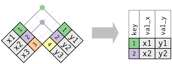
Bonus: Other dplyr join functions
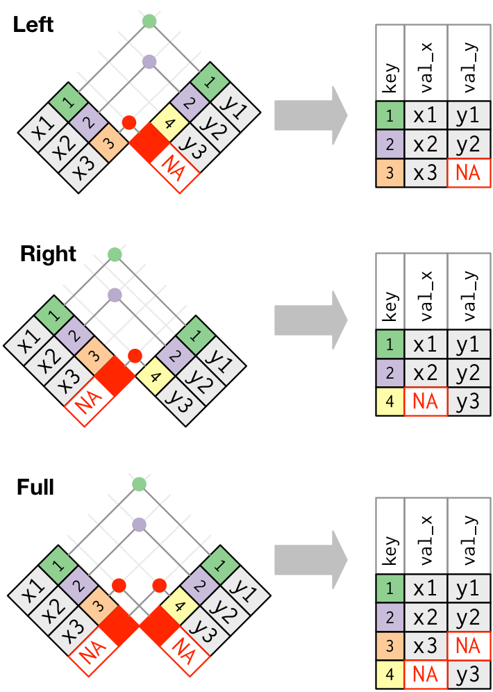
Outer joins and can be performed using
left_join(),right_join(), andfull_join(). In a “left join”, if the key is present in the left hand data frame, it will appear in the output, even if it is not found in the the right hand data frame. For a right join, the opposite is true. For a full join, all possible keys are included in the output data frame.
Let’s give the inner_join() function a try.
inner_join(gapminder_data, co2_emissions)
Joining, by = "country"
# A tibble: 1,188 × 8
country year pop continent lifeExp gdpPercap total_emission
<chr> <dbl> <dbl> <chr> <dbl> <dbl> <dbl>
1 Albania 1952 1282697 Europe 55.2 1601. 3825.
2 Albania 1957 1476505 Europe 59.3 1942. 3825.
3 Albania 1962 1728137 Europe 64.8 2313. 3825.
4 Albania 1967 1984060 Europe 66.2 2760. 3825.
5 Albania 1972 2263554 Europe 67.7 3313. 3825.
6 Albania 1977 2509048 Europe 68.9 3533. 3825.
7 Albania 1982 2780097 Europe 70.4 3631. 3825.
8 Albania 1987 3075321 Europe 72 3739. 3825.
9 Albania 1992 3326498 Europe 71.6 2497. 3825.
10 Albania 1997 3428038 Europe 73.0 3193. 3825.
# … with 1,178 more rows, and 1 more variable: per_capita_emission <dbl>
Do you see that we now have data from both data frames joined together in the same data frame? One thing to note about the output is that inner_join() tells us that that it joined by “country”. We can make this explicit using the “by” argument in the join functions
inner_join(gapminder_data, co2_emissions, by="country")
# A tibble: 1,188 × 8
country year pop continent lifeExp gdpPercap total_emission
<chr> <dbl> <dbl> <chr> <dbl> <dbl> <dbl>
1 Albania 1952 1282697 Europe 55.2 1601. 3825.
2 Albania 1957 1476505 Europe 59.3 1942. 3825.
3 Albania 1962 1728137 Europe 64.8 2313. 3825.
4 Albania 1967 1984060 Europe 66.2 2760. 3825.
5 Albania 1972 2263554 Europe 67.7 3313. 3825.
6 Albania 1977 2509048 Europe 68.9 3533. 3825.
7 Albania 1982 2780097 Europe 70.4 3631. 3825.
8 Albania 1987 3075321 Europe 72 3739. 3825.
9 Albania 1992 3326498 Europe 71.6 2497. 3825.
10 Albania 1997 3428038 Europe 73.0 3193. 3825.
# … with 1,178 more rows, and 1 more variable: per_capita_emission <dbl>
One thing to notice is that gapminder data had 25 rows, but the output of our join only had 21. Let’s investigate. It appears that there must have been countries in the gapminder data that did not appear in our co2_emissions data frame.
Let’s use anti_join() for this - this will show us the data for the keys on the left that are missing from the data frame on the right.
anti_join(gapminder_data, co2_emissions, by="country")
# A tibble: 516 × 6
country year pop continent lifeExp gdpPercap
<chr> <dbl> <dbl> <chr> <dbl> <dbl>
1 Afghanistan 1952 8425333 Asia 28.8 779.
2 Afghanistan 1957 9240934 Asia 30.3 821.
3 Afghanistan 1962 10267083 Asia 32.0 853.
4 Afghanistan 1967 11537966 Asia 34.0 836.
5 Afghanistan 1972 13079460 Asia 36.1 740.
6 Afghanistan 1977 14880372 Asia 38.4 786.
7 Afghanistan 1982 12881816 Asia 39.9 978.
8 Afghanistan 1987 13867957 Asia 40.8 852.
9 Afghanistan 1992 16317921 Asia 41.7 649.
10 Afghanistan 1997 22227415 Asia 41.8 635.
# … with 506 more rows
We can see that the co2_emissions data were missing for Bolivia, Puerto Rico, United States, and Venezuela.
If we look at the co2_emissions data with View(), we will see that Bolivia, United States, and Venezuela are called different things in the co2_emissions data frame. They’re called “Bolivia (Plurin. State of)”, “United States of America”, and “Venezuela (Boliv. Rep. of)”. Puerto Rico isn’t a country; it’s part of the United States. Using mutate() and recode(), we can re-import the co2_emissions data so that the country names for Bolivia, United States, and Venezuela, match those in the gapminder data.
co2_emissions <- read_csv("data/co2-un-data.csv", skip=2,
col_names=c("region", "country", "year",
"series", "value", "footnotes", "source")) %>%
select(country, year, series, value) %>%
mutate(series = recode(series, "Emissions (thousand metric tons of carbon dioxide)" = "total",
"Emissions per capita (metric tons of carbon dioxide)" = "per_capita")) %>%
pivot_wider(names_from=series, values_from=value) %>%
filter(year==2005) %>%
select(-year) %>%
mutate(country=recode(country,
"Bolivia (Plurin. State of)" = "Bolivia",
"United States of America" = "United States",
"Venezuela (Boliv. Rep. of)" = "Venezuela")
)
Rows: 2132 Columns: 7
── Column specification ─────────────────────────────────────────────────────────────────────────────────
Delimiter: ","
chr (4): country, series, footnotes, source
dbl (3): region, year, value
ℹ Use `spec()` to retrieve the full column specification for this data.
ℹ Specify the column types or set `show_col_types = FALSE` to quiet this message.
anti_join(gapminder_data, co2_emissions, by="country")
# A tibble: 480 × 6
country year pop continent lifeExp gdpPercap
<chr> <dbl> <dbl> <chr> <dbl> <dbl>
1 Afghanistan 1952 8425333 Asia 28.8 779.
2 Afghanistan 1957 9240934 Asia 30.3 821.
3 Afghanistan 1962 10267083 Asia 32.0 853.
4 Afghanistan 1967 11537966 Asia 34.0 836.
5 Afghanistan 1972 13079460 Asia 36.1 740.
6 Afghanistan 1977 14880372 Asia 38.4 786.
7 Afghanistan 1982 12881816 Asia 39.9 978.
8 Afghanistan 1987 13867957 Asia 40.8 852.
9 Afghanistan 1992 16317921 Asia 41.7 649.
10 Afghanistan 1997 22227415 Asia 41.8 635.
# … with 470 more rows
Now we see that our recode enabled the join for all countries in the gapminder, and we are left with Puerto Rico. In the next exercise, let’s recode Puerto Rico as United States in the gapminder data and then use group_by() and summarize() to aggregate the data; we’ll use the population data to weight the life expectancy and GDP values.
In the gapminder data, let’s recode Puerto Rico as United States.
gapminder_data <- read_csv("data/gapminder_data.csv") %>%
filter(year == 2007 & continent == "Americas") %>%
select(-year, -continent) %>%
mutate(country = recode(country, "Puerto Rico" = "United States"))
Rows: 1704 Columns: 6
── Column specification ─────────────────────────────────────────────────────────────────────────────────
Delimiter: ","
chr (2): country, continent
dbl (4): year, pop, lifeExp, gdpPercap
ℹ Use `spec()` to retrieve the full column specification for this data.
ℹ Specify the column types or set `show_col_types = FALSE` to quiet this message.
Now we have to group Puerto Rico and the US together, aggregating and calculating the data for all of the other columns. This is a little tricky - we will need a weighted average of lifeExp and gdpPercap.
gapminder_data <- read_csv("data/gapminder_data.csv") %>%
filter(year == 2007 & continent == "Americas") %>%
select(-year, -continent) %>%
mutate(country = recode(country, "Puerto Rico" = "United States")) %>%
group_by(country) %>%
summarize(lifeExp = sum(lifeExp * pop)/sum(pop),
gdpPercap = sum(gdpPercap * pop)/sum(pop),
pop = sum(pop)
)
Rows: 1704 Columns: 6
── Column specification ─────────────────────────────────────────────────────────────────────────────────
Delimiter: ","
chr (2): country, continent
dbl (4): year, pop, lifeExp, gdpPercap
ℹ Use `spec()` to retrieve the full column specification for this data.
ℹ Specify the column types or set `show_col_types = FALSE` to quiet this message.
Let’s check to see if it worked!
anti_join(gapminder_data, co2_emissions, by="country")
# A tibble: 0 × 4
# … with 4 variables: country <chr>, lifeExp <dbl>, gdpPercap <dbl>, pop <dbl>
Now our anti_join() returns an empty data frame, which tells us that we have reconciled all of the keys from the gapminder data with the data in the co2_emissions data frame.
Finally, let’s use the inner_join() to create a new data frame:
gapminder_co2 <- inner_join(gapminder_data, co2_emissions, by="country")
One last thing! What if we’re interested in distinguishing between countries in North America and South America? We want to create two groups - Canada, the United States, and Mexico in one and the other countries in another.
We can create a grouping variable using mutate() combined with an if_else() function - a very useful pairing.
gapminder_co2 %>%
mutate(region = if_else(country == "Canada" | country == "United States" | country == "Mexico", "north", "south"))
# A tibble: 24 × 7
country lifeExp gdpPercap pop total per_capita region
<chr> <dbl> <dbl> <dbl> <dbl> <dbl> <chr>
1 Argentina 75.3 12779. 40301927 149476. 3.82 south
2 Bolivia 65.6 3822. 9119152 8976. 0.984 south
3 Brazil 72.4 9066. 190010647 311624. 1.67 south
4 Canada 80.7 36319. 33390141 540431. 16.8 north
5 Chile 78.6 13172. 16284741 54435. 3.34 south
6 Colombia 72.9 7007. 44227550 53585. 1.24 south
7 Costa Rica 78.8 9645. 4133884 5463. 1.29 south
8 Cuba 78.3 8948. 11416987 25051. 2.22 south
9 Dominican Republic 72.2 6025. 9319622 17522. 1.90 south
10 Ecuador 75.0 6873. 13755680 23927. 1.74 south
# … with 14 more rows
Let’s look at the output - see how the Canada, US, and Mexico rows are all labeled as “north” and everything else is labeled as “south”
We have reached our data cleaning goals! One of the best aspects of doing all of these steps coded in R is that our efforts are reproducible, and the raw data is maintained. With good documentation of data cleaning and analysis steps, we could easily share our work with another researcher who would be able to repeat what we’ve done. However, it’s also nice to have a saved csv copy of our clean data. That way we can access it later without needing to redo our data cleaning, and we can also share the cleaned data with collaborators. To save our dataframe, we’ll use write_csv().
write_csv(gapminder_co2, "data/gapminder_co2.csv")
Great - Now we can move on to the analysis!
Analyzing combined data
For our analysis, we have two questions we’d like to answer. First, is there a relationship between the GDP of a country and the amount of CO2 emitted (per capita)? Second, Canada, the United States, and Mexico account for nearly half of the population of the Americas. What percent of the total CO2 production do they account for?
To answer the first question, we’ll plot the CO2 emitted (on a per capita basis) against the GDP (on a per capita basis) using a scatter plot:
ggplot(gapminder_co2, aes(x=gdpPercap, y=per_capita)) +
geom_point() +
labs(x="GDP (per capita)",
y="CO2 emitted (per capita)",
title="There is a strong association between a nation's GDP \nand the amount of CO2 it produces"
)

Tip: Notice we used the \n in our title to get a new line to prevent it from getting cut off.
To help clarify the association, we can add a fit line through the data using geom_smooth()
ggplot(gapminder_co2, aes(x=gdpPercap, y=per_capita)) +
geom_point() +
labs(x="GDP (per capita)",
y="CO2 emitted (per capita)",
title="There is a strong association between a nation's GDP \nand the amount of CO2 it produces"
) +
geom_smooth()
`geom_smooth()` using method = 'loess' and formula 'y ~ x'

We can force the line to be straight using method="lm" as an argument to geom_smooth
ggplot(gapminder_co2, aes(x=gdpPercap, y=per_capita)) +
geom_point() +
labs(x="GDP (per capita)",
y="CO2 emitted (per capita)",
title="There is a strong association between a nation's GDP \nand the amount of CO2 it produces"
) +
geom_smooth(method="lm")
`geom_smooth()` using formula 'y ~ x'

To answer our first question, as the title of our plot indicates there is indeed a strong association between a nation’s GDP and the amount of CO2 it produces.
For the second question, we want to create two groups - Canada, the United States, and Mexico in one and the other countries in another.
We can create a grouping variable using mutate() combined with an if_else() function - a very useful pairing.
gapminder_co2 %>%
mutate(region = if_else(country == "Canada" | country == "United States" | country == "Mexico", "north", "south"))
# A tibble: 24 × 7
country lifeExp gdpPercap pop total per_capita region
<chr> <dbl> <dbl> <dbl> <dbl> <dbl> <chr>
1 Argentina 75.3 12779. 40301927 149476. 3.82 south
2 Bolivia 65.6 3822. 9119152 8976. 0.984 south
3 Brazil 72.4 9066. 190010647 311624. 1.67 south
4 Canada 80.7 36319. 33390141 540431. 16.8 north
5 Chile 78.6 13172. 16284741 54435. 3.34 south
6 Colombia 72.9 7007. 44227550 53585. 1.24 south
7 Costa Rica 78.8 9645. 4133884 5463. 1.29 south
8 Cuba 78.3 8948. 11416987 25051. 2.22 south
9 Dominican Republic 72.2 6025. 9319622 17522. 1.90 south
10 Ecuador 75.0 6873. 13755680 23927. 1.74 south
# … with 14 more rows
Now we can use this column to repeat our group_by() and summarize() steps
gapminder_co2 %>%
mutate(region = if_else(country == "Canada" |
country == "United States" |
country == "Mexico", "north", "south")) %>%
group_by(region) %>%
summarize(sumtotal = sum(total),
sumpop = sum(pop))
# A tibble: 2 × 3
region sumtotal sumpop
<chr> <dbl> <dbl>
1 north 6656037. 447173470
2 south 889332. 451697714
The if_else() statement reads like, “if country equals “Canada” OR | “United states” OR “Mexico”, the new variable region should be “north”, else “south””. It’s worth exploring logical operators for “or” |, “and” &&, and “not” !, which opens up a great deal of possibilities for writing code to do what you want.
We see that although Canada, the United States, and Mexico account for close to half the population of the Americas, they account for 88% of the CO2 emitted. We just did this math quickly by plugging the numbers from our table into the console to get the percentages. Can we make that a little more reproducible by calculating percentages for population (pop) and total emissions (total) into our data before summarizing?
Finishing with Git and GitHub
Awesome work! Let’s make sure it doesn’t go to waste. Time to add, commit, and push our changes to GitHub again - do you remember how?
changing directories
Print your current working directory and list the items in the directory to check where you are. If you are not in the un-report directory, navigate there.
Solution:
pwd ls cd ~/Desktop/un-report ls
reviewing git and GitHub
Pull to make sure our local repository is up to date. Then add, commit, and push your commits to GitHub. Don’t forget to check your git status periodically to make sure everything is going as expected!
Solution:
git status git pull git status git add "data-analysis.R" git status git commit -m "Create data analysis file" git status git log --online git push git status
Bonus
Bonus content
Sort data with arrange()
The arrange() function allows us to sort our data by some value. Let’s use the gapminder_data dataframe. We will take the average value for each continent in 2007 and then sort it so the continents with the longest life expectancy are on top. Which continent might you guess has be highest life expectancy before running the code?
The helper function ends_with() can help us here.
gapminder_data %>%
filter(year==2007) %>%
group_by(continent) %>%
summarise(average= mean(lifeExp)) %>%
arrange(desc(average))
Error: Problem with `filter()` input `..1`.
ℹ Input `..1` is `year == 2007`.
✖ object 'year' not found
Notice there that we can use the column created the in the summarize() step (“average”) later in the arrange() step. We also use the desc() function here to sort the values in a descending order so the largest values are on top. The default is to put the smallest values on top.
Bonus exercises
Calculating percent
What percentage of the population and CO2 emissions in the Americas does the United States make up? What percentage of the population and CO2 emission does North America make up?
Solution
Create a new variable using
mutate()that calculates percentages for the pop and total variables.gapminder_co2 %>% mutate(region = if_else(country == "Canada" | country == "United States" | country == "Mexico", "north", "south")) %>% mutate(totalPercent = total/sum(total)*100, popPercent = pop/sum(pop)*100)# A tibble: 24 × 9 country lifeExp gdpPercap pop total per_capita region totalPercent <chr> <dbl> <dbl> <dbl> <dbl> <dbl> <chr> <dbl> 1 Argentina 75.3 12779. 4.03e7 1.49e5 3.82 south 1.98 2 Bolivia 65.6 3822. 9.12e6 8.98e3 0.984 south 0.119 3 Brazil 72.4 9066. 1.90e8 3.12e5 1.67 south 4.13 4 Canada 80.7 36319. 3.34e7 5.40e5 16.8 north 7.16 5 Chile 78.6 13172. 1.63e7 5.44e4 3.34 south 0.721 6 Colombia 72.9 7007. 4.42e7 5.36e4 1.24 south 0.710 7 Costa Rica 78.8 9645. 4.13e6 5.46e3 1.29 south 0.0724 8 Cuba 78.3 8948. 1.14e7 2.51e4 2.22 south 0.332 9 Dominican Re… 72.2 6025. 9.32e6 1.75e4 1.90 south 0.232 10 Ecuador 75.0 6873. 1.38e7 2.39e4 1.74 south 0.317 # … with 14 more rows, and 1 more variable: popPercent <dbl>This table shows that the United states makes up 33% of the population of the Americas, but accounts for 77% of total emissions. Now let’s take a look at population and emission for the two different continents:
gapminder_co2 %>% mutate(region = if_else(country == "Canada" | country == "United States" | country == "Mexico", "north", "south")) %>% mutate(totalPercent = total/sum(total)*100, popPercent = pop/sum(pop)*100) %>% group_by(region) %>% summarize(sumTotalPercent = sum(totalPercent), sumPopPercent = sum(popPercent))# A tibble: 2 × 3 region sumTotalPercent sumPopPercent <chr> <dbl> <dbl> 1 north 88.2 49.7 2 south 11.8 50.3
CO2 bar plot
Create a bar plot of the percent of emissions for each country, colored by north and south america (HINT: use geom_col())
Solution
gapminder_co2 %>% ggplot(aes(x = country, y = total_emissionsPercent, fill = region)) +
geom_col()
Error in FUN(X[[i]], ...): object 'total_emissionsPercent' not found
Now rotate the x-labels by 90 degrees (if you don’t remember how, google it again or look at our code from the ggplot lesson)
Solution
gapminder_co2 %>% ggplot(aes(x = country, y = total_emissionsPercent, fill = region)) +
geom_col() +
theme(axis.text.x = element_text(angle = 90, hjust = 1, vjust = 0.5))
Error in FUN(X[[i]], ...): object 'total_emissionsPercent' not found
Reorder the bars in descending order. Hint: try Googling how to use the
reorder()function with ggplot.Solution
gapminder_co2 %>% ggplot(aes(x = reorder(country, - total_emissionsPercent), y = total_emissionsPercent, fill = region)) +
geom_col() +
theme(axis.text.x = element_text(angle = 90, hjust = 1, vjust = 0.5))
Error in tapply(X = X, INDEX = x, FUN = FUN, ...): object 'total_emissionsPercent' not found
Practice making it look pretty!


low emissions
Find the 3 countries with lowest per capita emissions. Hint: use the
arrange()function.Solution
gapminder_co2 %>% arrange(per_capita_emissions)Error: arrange() failed at implicit mutate() step. * Problem with `mutate()` column `..1`. ℹ `..1 = per_capita_emissions`. ✖ object 'per_capita_emissions' not foundCreate a bar chart for the per capita emissions for just those three countries.
Solution
gapminder_co2 %>% filter(country == "Haiti" | country == "Paraguay" | country == "Nicaragua") %>%
ggplot(aes(x = country, y = per_capita_emissions)) +
geom_col()
Error in FUN(X[[i]], ...): object 'per_capita_emissions' not found
Reorder them in descending order. Hint: use the
reorder()function.Solution
gapminder_co2 %>% filter(country == "Haiti" | country == "Paraguay" | country == "Nicaragua") %>%
ggplot(aes(x = reorder(country, - per_capita_emissions), y = per_capita_emissions)) +
geom_col()
Error in tapply(X = X, INDEX = x, FUN = FUN, ...): object 'per_capita_emissions' not found


Key Points
Package loading is an important first step in preparing an R environment.
Data analsyis in R facilitates reproducible research.
There are many useful functions in the
tidyversepackages that can aid in data analysis.Assessing data source and structure is an important first step in analysis.
Preparing data for analysis can take significant effort and planning.